Simulating Lorenz attractor in Sinumerik

A while back I learned about the Lorenz attractor that was the result of trying to model the weather, the interesting property of the Lorenz attractor (and thus also the weather) is that given different initial conditions, the systems trajectories varies a lot and is for long time horizons basically impossible to predict.

I really like the example by Sebastien Gros in a lecture on numerical optimal control, where the chaotic properties of the systems basically makes it almost impossible to find a optimal control input for a long time horizon.

The Lorenz attractor is maybe more known by its butterfly like 3D-graph. But since this is only a standard plot, I thought it would be cool to implement it on a real world 3D-plotter, or as other may call it a CNC-machine.

In this post I will go into numerical integration a.k.a. simulating dynamical systems, and touch briefly on Sinumerik CNC programming. A combo that I’ve never seen before and should hopefully result in an interesting read.

Lorenz attractor

The Lorenz attractor is a dynamical system with 3 states, where their derivatives are defined according to

\[\begin{align} \frac{dx}{dt} &= \sigma (y-x) \\ \frac{dy}{dt} &= x(\rho - z) - y \\ \frac{dz}{dt} &= xy - \beta z \end{align}\]

and one can use the following parameters to yield the classic butterfly curve

\[\sigma = 10, \quad \beta = 8/3, \quad \rho=28 .\]

Simulation of dynamical systems

The standard setup for simulating any dynamical system starts with the system equation

\[\dot x_s = f(x_s,u),\]

were \(x_s\) is the state vector (don’t mix it up with \(x\) in the Lorenz system) and \(u\) in the control input signal. For our Lorenz system we don’t have an input signal, so the system will only depend on its state.

\[\dot x_s = f(x_s) = \begin{bmatrix} \sigma (y-x) \\ x(\rho - z) - y \\ xy - \beta z \end{bmatrix}\]

and the state vector is defined as

\[x_s = \begin{bmatrix} x \\ y\\ z \end{bmatrix}\]

When the system equation are given, the goal is that given an initial state \(x_0\) (and optionally a time series of the control signal \(u\)) and a time step, to create a time series of the state trajectory. Or more simply, given \(f\), \(x_0\) and \(\Delta T\) compute the time series signal \(x_s [0] ... x_s[N]\) that represent how the system states changes.

Forward Euler

When I first learnt about numerical integration/system simulation, I started with the Forward Euler method, which I think is a nice introduction to the problem and the general difficulties with simulation.

The idea behind Forward Euler is that the derivative is assumed to be constant over each time step, that means that the state at step \(k\) is computed as

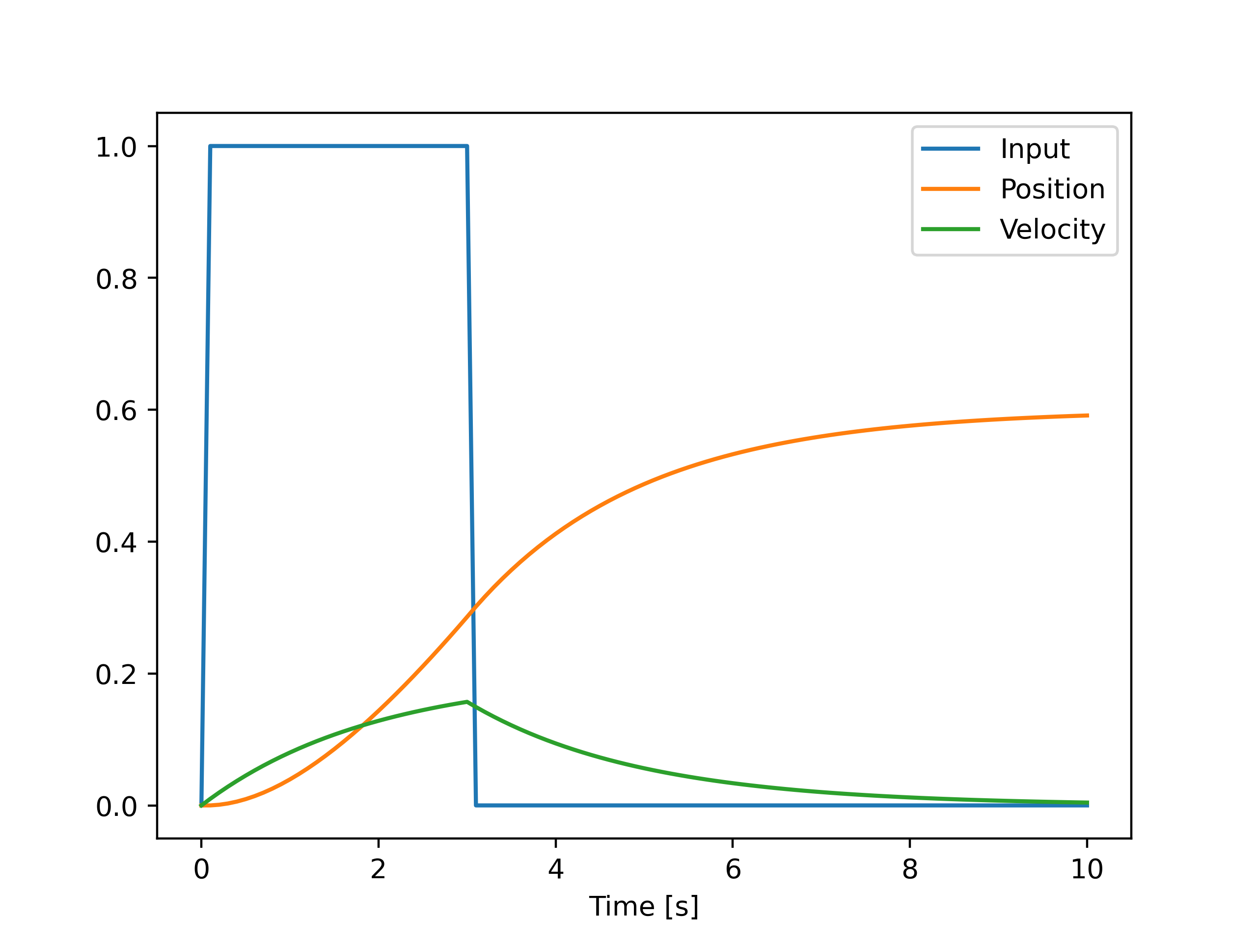
\[x_s[k] = x_s[k-1] + f(x_s[k-1])\Delta T\]

In the following code snippet I implemented a simple simulation of a mass on a cart where the position of the cart is \(p\), and the the acceleration of the cart is given as

\[\ddot p = \frac{u - \dot p d}{M}\]

where $d$ is viscous friction coefficient, the cart starts at position 0 at a standstill and for the first 3 seconds, a force of 1N is applied.

import numpy as np 
import matplotlib.pyplot as plt 

def f(x,u):
    # System equations for a single mass system
    # Extract state vector
    p = x[0] # position
    v = x[1] # speed 

    # System parameters
    M = 10
    d = 5

    acc = (u -d*v)*1/M
    dot_x = np.array([v,acc])
    return dot_x

def simulation():

    Tf = 10 
    dt = 0.1
    N = int(np.ceil(Tf/dt))
    t_vec = np.linspace(0,Tf,N+1)

    x0 = np.array([0,0])

    Us = [0]
    Xs = [x0]

    for i in range(N):
        ti = t_vec[i]

        u = 0
        if ti < 3:
            u = 1
        Us.append(u)

        dot_x = f(Xs[i],u)

        X_plus = Xs[i] + dot_x*dt 
        Xs.append(X_plus)

    Xs = np.array(Xs)
    position = Xs[:,0]
    velocity = Xs[:,1]

    plt.plot(t_vec,Us,label='Input')
    plt.plot(t_vec,position,label='Position')
    plt.plot(t_vec,velocity,label='Velocity')
    plt.legend()
    plt.xlabel('Time [s]')
    plt.show()

if __name__ == '__main__':
    simulation()

The resulting state trajectory is shown in the figure below.

Runge-Kutta

Even if Forward Euler is easy to understand it does have one big drawback, in order to yield accurate results, it requires really small timesteps, i.e. \(\Delta T\), this means more computation is needed and thus longer time to simulate. In order to simulate systems more accurate without needing small timesteps, the Runge-Kutta method was developed, more info can be found on Wikipedia.

Here I will use the Runge-Kutta method of 4th order, often denoted RK4.

At time-step \(k\), the following coefficients are computed

\[\begin{align} k_1 &= f(x_s[k],t[k]) \\ k_2 &= f(x_s[k] + \Delta T \frac{k_1}{2},t[k] + \frac{h}{2}) \\ k_3 &= f(x_s[k] + \Delta T \frac{k_2}{2},t[k] + \frac{h}{2}) \\ k_4 &= f(x_s[k] + \Delta T k_3,t) \end{align}\]

and they are then used to compute the next step

\[x_s[k+1] = x_s[k] + \frac{1}{6}\Delta T(k1 + 2 k_2 + 2k_3 + k_4).\]

Even if there is more computations required in the RK method, it still outweighs the Newton method for larger systems and where smaller error tolerances is required.

In the following code snippet I show how to use RK4 to solve for the state trajectory of the Lorenz system.

import matplotlib.pyplot as plt 
from mpl_toolkits.mplot3d import Axes3D
import numpy as np 

def lorenz(X):
    x = X[0]
    y = X[1]
    z = X[2]

    sigma = 10 
    beta = 8/3
    rho = 28

    dx = sigma * (y-x)
    dy = x*(rho - z) - y 
    dz = x*y - beta*z

    return np.array([dx,dy,dz])

def ruku4(X,h):
    k_1 = lorenz(X)
    k_2 = lorenz(X + k_1*h/2)
    k_3 = lorenz(X + k_2*h/2)
    k_4 = lorenz(X + h*k_3)

    deltaX = 1/6*h*(k_1 + 2*k_2 + 2*k_3 + k_4)
    x_plus = X + deltaX 

    return x_plus

def main():

    N = 200
    X = np.array([-1,0,22])
    Xs = np.array([X])

    h = 0.02

    fig = plt.figure()

    for i in range(N):

        if i%10==0:
            print(i)

        X = ruku4(X,h)
        Xs = np.vstack((Xs,X))
    
        plt.clf()
        ax = fig.add_subplot(111, projection='3d')
        ax.plot(Xs[:,0],Xs[:,1],Xs[:,2])
        
        ax.set_xlim(-20,20)
        ax.set_ylim(-25,25)
        ax.set_zlim(5,45)

        #plt.savefig(f'pythonScreenshots/plot_{i}.png')

    ax.set_xlabel('X')
    ax.set_ylabel('Y')
    ax.set_zlabel('Z')
    plt.show()

if __name__ == '__main__':
    main()

Sinumerik implementation

In order to simulate the Lorenz system on a Sinumerik CNC-machine, I implemented the lorenz equation and the RK4 function. Below are the main program shown and also a GIF from the Sinutrain simulator.

If you are interested in the Sinumerik code, I would refer to the github repo.

DEF REAL STATE[3], DELTA, STATE_PLUS[3]
DEF INT INK,NR_POINTS

EXTERN LORENZ_RUKU4(VAR REAL[3], VAR REAL[3], REAL)

; Simulation params
NR_POINTS = 1500
DELTA = 0.02

; Initial condition
STATE[0] = -1;1
STATE[1] = 0;1
STATE[2] = 22;30

G94 F=100
G0 X=STATE[0] Y=STATE[1] Z=STATE[2]
;M0
STOPRE
FOR INK=0 TO NR_POINTS
	LORENZ_RUKU4(STATE,STATE_PLUS,DELTA)
	G1 X=STATE_PLUS[0] Y=STATE_PLUS[1] Z=STATE_PLUS[2]
	;M0
    ;STOPRE
	STATE[0] = STATE_PLUS[0]
	STATE[1] = STATE_PLUS[1]
	STATE[2] = STATE_PLUS[2]
ENDFOR

M30

That’s all for this time, thanks for reading! And as you might have noticed the Sinumerik implementation is from last year… and that’s sometimes how it is. Hopefully the next post will come sooner.